These results, of mother cells ever increasing and giving birth to larger daughters, lead to the intuition that this model might generate stable and continuous size distributions on the population level.
The model we used has been written in a format similar to that used by
Gyllenberg (1986). The model Gyllenberg put forward differs from ours on
three main features. First, in his model the yeast cell is characterized by
mass only, while we additionally characterize the cell with chemical
species involved in the division cycle. Secondly, we model the START
transition as a purely deterministic event while Gyllenberg uses a
stochastic event based on cell size. Thirdly, Gyllenberg considers the
length of the budded period constant for all scar classes, while in our
model this period depends on the state at which a cell enters the budded
period and is therefore not necessarily constant. For his model Gyllenberg
has proved the convergence to stable scar and size distributions for certain
conditions on growth and birth rates. Even in the absence of a stochastic
START transition this convergence takes place in Gyllenberg's model as long
as the cell cycle lengths for the various scar classes are not
commensurable, i.e. there does not exist a ![]() such that the length of
the cell cycle for each scar class is an integral multiple of
such that the length of
the cell cycle for each scar class is an integral multiple of ![]() .
.
Our model essentially matches the latter case of Gyllenbergs model. However, in our case (in contrast to Gyllenberg model) cells belonging to one scar class do not all have the same cell cycle length. For this reason we could not simply make use of the proof given by Gyllenberg. We therefore put forward the following conjecture:

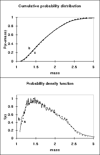
Figure:3 Typical results for
the steady state size distribution obtained by
a) numerically solving the PDE (14) (dashed line) and b) a solution of the finite
number approach after a ![]() min run (solid line). Note that the distribution of the
finite number approach is slightly wider than that obtained by numerically
solving the pde. The results are independent of the initial state of the
population. For parameter values see Fig. 2.
min run (solid line). Note that the distribution of the
finite number approach is slightly wider than that obtained by numerically
solving the pde. The results are independent of the initial state of the
population. For parameter values see Fig. 2.

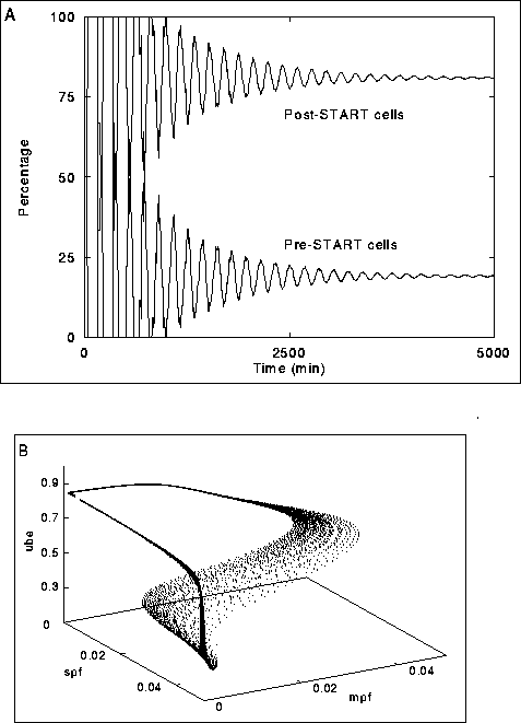
Figure:4 The numerical solution of the PDE
(14) using the escalator boxcar train method (De Roos et al. 1990):
A) Convergence of the solution represented by the fractions of pre- and post-START cells.
B) Trajectories (cf. Fig. 2) at steady state.
For parameter values see Fig. 2.
Although we are not able to prove this statement, we would like to present
numerical results that we obtained by two different approaches to support
it. In the first approach, we used the escalator boxcar train method (de
Roos et al. 1990) for solving the partial differential equations
numerically. Since the state space and the boundaries of the state space
have high dimensions, a numerical solution of the structured model requires
lots of computer memory and processor time. Our simulations give rise to
stable distributions (Fig. 3, Fig. 4A), but,
due to the limitation in grid
size, these distributions may not accurately reflect the true distribution.
Figure 4B shows a typical state of the model after a long run which started
with a population consisting of smallest cells only. Clearly one can see the
trajectories which cells follow through state space, and the result of
the coarseness of the grid used for the boundary ( ![]() ) in solving
the PDE.
) in solving
the PDE.
In the second approach (referred to as finite number approach), we took
advantage of the fact that the model consists of a set of linear partial
differential equations and therefore the trajectories for cells born with
the same initial state are identical. We constructed
a lookup table for a set of points in ![]() relating the state at
birth of each cell to its cell cycle length and to the states at birth of
its two descendants (the daughter progeny and the resulting mother). The
relation was obtained by numerically solving the ODE (1) for
each set of initial conditions in the table and linear interpolation was
used for initial conditions that did not match precisely to one of the
entries in the table. In a branching process we kept track of the lineages
(i.e., we followed each cell and all its descendants, mothers and daughters)
of a fixed number of cells H at time 0 up to some time S. After each
division, the lookup table was used to generate the fate of the new
offspring. After S time units, we thinned the population back by randomly
choosing H individuals and then continued the lineages of those H
individuals up to the next S time units. This process was repeated until
the distribution more or less settled. The final distributions did not
depend on the choice of the initial H individuals. Unfortunately due to
the random thinning process the resulting distributions (Fig. 3) are random
variables as well and can not be used to show a convergence to a stable
distribution.
relating the state at
birth of each cell to its cell cycle length and to the states at birth of
its two descendants (the daughter progeny and the resulting mother). The
relation was obtained by numerically solving the ODE (1) for
each set of initial conditions in the table and linear interpolation was
used for initial conditions that did not match precisely to one of the
entries in the table. In a branching process we kept track of the lineages
(i.e., we followed each cell and all its descendants, mothers and daughters)
of a fixed number of cells H at time 0 up to some time S. After each
division, the lookup table was used to generate the fate of the new
offspring. After S time units, we thinned the population back by randomly
choosing H individuals and then continued the lineages of those H
individuals up to the next S time units. This process was repeated until
the distribution more or less settled. The final distributions did not
depend on the choice of the initial H individuals. Unfortunately due to
the random thinning process the resulting distributions (Fig. 3) are random
variables as well and can not be used to show a convergence to a stable
distribution.

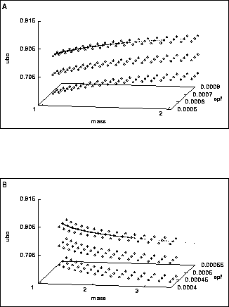
Figure:5 Concentration of the states at birth of daughters (A) and mothers (B)
on lines in the hyper surface ![]() (Eq. 3). The squares denote
entries in the lookup table, all of the entries serving as the initial condition in this
simulation. Interpolation or extrapolation is used to
obtain new states at birth. The line of dots resembles the population (about
25,000 cells) which was present after a simulation for
(Eq. 3). The squares denote
entries in the lookup table, all of the entries serving as the initial condition in this
simulation. Interpolation or extrapolation is used to
obtain new states at birth. The line of dots resembles the population (about
25,000 cells) which was present after a simulation for ![]() minutes. The population
concentrates on the line formed by those entries which are part of the lineage of
the smallest cell in a culture in balanced growth (see main text).
Simulations started with other initial conditions do not differ from the result obtained
in this particular example.
For parameter values see 2.
minutes. The population
concentrates on the line formed by those entries which are part of the lineage of
the smallest cell in a culture in balanced growth (see main text).
Simulations started with other initial conditions do not differ from the result obtained
in this particular example.
For parameter values see 2.
Figure 5 shows that the birth states are concentrating on two lines through the 4 dimensional state space, one for the mother cells (Fig. 5A) and one for the daughters (Fig. 4B). Conditions (9) and (10) are boundaries on a 3-dimensional hyper surface, but the dynamics of growth and division compresses this 3-dimensional set to a 1-dimensional set.
The combination of the results from both approaches supports our conjecture.
In Fig. 3 we can see that the distributions of the two different numerical
approaches do not differ much. The distribution generated by the finite
number approach is slightly broader than the distribution obtained by
solving the PDEs numerically. Numerical solutions of the PDEs approach a
stable size distribution despite the coarse grid size, whereas there is no
grid size limitation in the finite number approach. Furthermore, the finite
number approach shows that the newborn cells fill a 1-dimensional dense set
in ![]() (Fig 5).
(Fig 5).

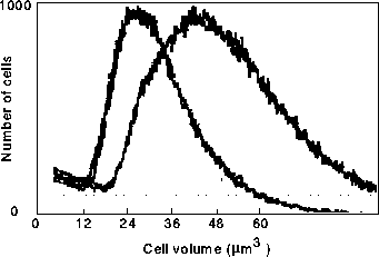
Figure:6 Experimental volume distributions for two different cell lines (Nash
at al. 1988, printed with permission of Oxford University Press). Note that the relative width (volume at line intersection /
minimal volume) of the distributions is about 5 for each cell line, while in
our numerical approaches the relative width is only 2.5 (Fig.3 ).
The line intersection
is arbitrarily set to 10 % of the hight of the distribution.
Experiments (Nash et al. 1988) show that the shape of the actual distributions is reasonably similar to what we find (Fig. 6). However the relative width of actual size distribution is about two-fold larger than the ones we obtain (Fig.3). For parameters in this calculations, division cycles cease when cells are born with a size about 20 times the smallest birth size. The cycles at larger sizes can only occur far in the mother lineage of zero scar cells ( The cycle in Fig. 4B was the 81st generation as mother of the smallest cell). The reason most of the weight in the distribution is below three times the minimal cell size is that with each consecutive mother generation the chance that this mother is still being present in the culture is decreasing exponentially, and so large mothers hardly contribute to the cell population (cf. Gyllenberg, 1986, Hartwell & Unger, 1977). In order to increase the width of the theoretical distribution more variation in the cell cycle length of the lower generation cells in response to small changes in mass is needed. Within the current dynamical setting, we were not able to find parameter sets which would allow for this.