In this section we derive the transformation equations (4,7, and 8). Let us start from the output function
For the uniform distribution 11 over [t-h,t]
![]()
and
![]()
from which follows eq. (7). For the exponential distribution
![]()
and
from which follows eq. (8).
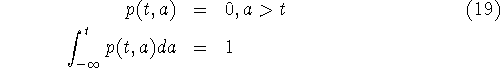
We are left to derive the translation rule (4) for method 1. We again start from the output function
in which
and f(a) is a sufficiently smooth function.
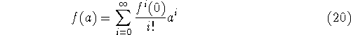
Our goal is to find f(a) from the experimental time series F(t) and experimental information about the distribution p(t,a). We proceed by Taylor expansion of the function f(a) around age 0,
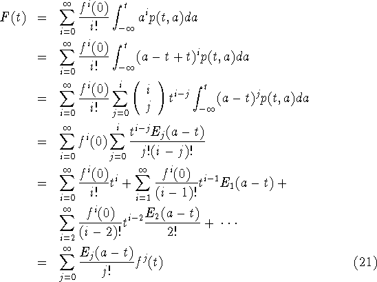
Substitution in (18) results in
where
![]()
is the expectation of ![]() over distribution p(t,a) at time t.
Series (21) gives us the dependence of F on f, but our
problem is to obtain the inverse. As a start we write
over distribution p(t,a) at time t.
Series (21) gives us the dependence of F on f, but our
problem is to obtain the inverse. As a start we write
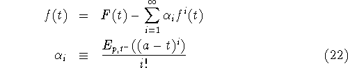
Because of our assumption that cells move deterministically through state
space p(t,a) is time invariant, i.e. ![]() . In
this case the moments
. In
this case the moments ![]() are independent of t,
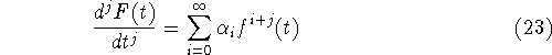
and therefore the derivatives of F with time are given by
are independent of t,
and therefore the derivatives of F with time are given by
Combining (23) and (22) we get the wanted transformation rule (4).
Equations (4) and (5) now fully describe f(t) as a function of the experimental information F(t) and p(t,a). The derivatives of F(t) with respect to time have to be obtained numerically. Some truncation of (4) is therefore likely to happen, which makes it necessary to show that the sum in (4) converges. We suspect that for distributions for which all higher moments do exist convergence is there since we have nothing but rewritten the converging Taylor series (20) as (4), however this still needs to be proved.