In section 3 the synchronization methods were used on experimental output where the underlying individual output function is not known. To get some insight in the validity of the methods we here apply the methods on theoretical output from a known individual output function. We will show that the methods do very well when applied to output generated by the assumptions they were derived for, but that sever mistakes can be made when applied to the output generated from the wrong set of assumptions. However, the example here is a worst case scenario.
For all the theoretical examples we assume that the individual output function is
![]()
As a first example for both method 1 and 2 we choose the exponential distribution (14). The output function then reads
where ![]() for method 1 or
for method 1 or ![]() for method 2. The
inverse function equals
for method 2. The
inverse function equals
A second distribution we use for method 1 is a variation of the ![]() -distribution
-distribution ![]() (9). In this case the
output function and its inverse read
(9). In this case the
output function and its inverse read
For method 2 we use a uniform distribution (11) for the probability of passing some crucial state in the cell cycle for method 2 is the resulting in
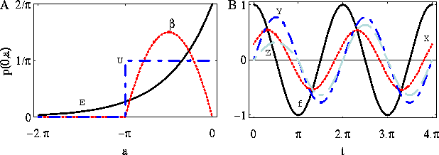
In figure 6 f(a), ![]() ,
and
,
and ![]() are plotted.
are plotted.

Figure 6: The probability distributions (A) ![]() ,
, ![]() ,
, ![]() and
(B) the function f(t)=cos(t) and its variation distorted outputs
and
(B) the function f(t)=cos(t) and its variation distorted outputs ![]() .)
.)
Suppose we have a series of observed values ![]() of an output function F(t). How close do we get to f(a) if we apply the
inverse functions on this series? In the case of the exponential
distribution and the uniform distribution in either model 1 or 2 we need
estimates of the first derivative only. Derivatives are found numerically by
differentiating spline functions running through the data points (see
appendix C). Finding f(t) from the series
of an output function F(t). How close do we get to f(a) if we apply the
inverse functions on this series? In the case of the exponential
distribution and the uniform distribution in either model 1 or 2 we need
estimates of the first derivative only. Derivatives are found numerically by
differentiating spline functions running through the data points (see
appendix C). Finding f(t) from the series ![]() , and
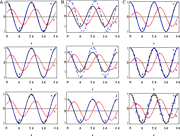
, and ![]() is (not surprisingly) very accurate (fig. 7-A). In
case of the
is (not surprisingly) very accurate (fig. 7-A). In
case of the ![]() -distribution, method 1 requires an infinite series of
derivatives of Y. The series
-distribution, method 1 requires an infinite series of
derivatives of Y. The series ![]() can at most be described by a
can at most be described by a ![]() order polynomial, so truncation of the series of
derivatives is unavoidable. However a sufficient approximation of the
original function does not require estimation of all the derivatives as is
seen in fig. 7-B. This figure also shows that having more
data points does not necessarily improve the approximation, but it is rather
the quality of estimating the higher derivatives of the output function
which make the approximation better. It is only after having the right
number of derivatives (in all our computations a third order approximation
turned out to be sufficient) that more data points result in a better fit
(results not shown).
order polynomial, so truncation of the series of
derivatives is unavoidable. However a sufficient approximation of the
original function does not require estimation of all the derivatives as is
seen in fig. 7-B. This figure also shows that having more
data points does not necessarily improve the approximation, but it is rather
the quality of estimating the higher derivatives of the output function
which make the approximation better. It is only after having the right
number of derivatives (in all our computations a third order approximation
turned out to be sufficient) that more data points result in a better fit
(results not shown).

Figure 7: Results of retrieving f from a series ![]() on the interval
[0,4/pi] A) x(t) from
on the interval
[0,4/pi] A) x(t) from ![]() using method 1. B) y(t) from Y(t) using method 1. C) z(t) from Z(t) using method 2. In the upper,
middle, and lower graphs the interval was split up in 64, 32 and 16
intervals respectively and a spline function consisting of respectively
linear, quadratic, third order elements was used to determine the
derivatives required.
using method 1. B) y(t) from Y(t) using method 1. C) z(t) from Z(t) using method 2. In the upper,
middle, and lower graphs the interval was split up in 64, 32 and 16
intervals respectively and a spline function consisting of respectively
linear, quadratic, third order elements was used to determine the
derivatives required.
In a real experiment we have to judge whether method 1 or method 2 applies.
We used the examples with the uniform distributions to see what mistakes we
make if we use the wrong inverse function on the output function. One
mistake we can make is using method 2 to obtain a synchronized output
function ![]() from data generated by the output function underlying
method 1, i.e. we apply (29) to Y(t) with
from data generated by the output function underlying
method 1, i.e. we apply (29) to Y(t) with ![]() (
( ![]() ) to obtain
) to obtain ![]() as an estimate of y(t). So we have
as an estimate of y(t). So we have

Note that Y(0) = ![]() is non zero for most h. Data
generated by an output function underlying method 1 (17)
necessarily has a zero value at t=0. Therefore we can not apply eq. (29) directly. If in addition we assume that all cells in the culture
have a constant output Y(0) in all phases in its life, applying eq. (29) results in
is non zero for most h. Data
generated by an output function underlying method 1 (17)
necessarily has a zero value at t=0. Therefore we can not apply eq. (29) directly. If in addition we assume that all cells in the culture
have a constant output Y(0) in all phases in its life, applying eq. (29) results in
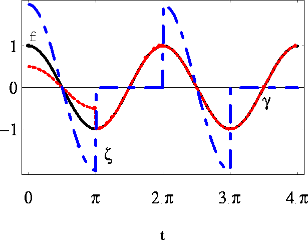
Figure 8 shows that ![]() is very different from f(t)
for the particular choice
is very different from f(t)
for the particular choice ![]() .
.

Figure 8: Results of retrieving f using the wrong synchronization method.
For explanation see text.
Another mistake is evident if we use method 1 to synchronize data generated
by an output function underlying model 2, i.e. we apply (27) to Z(t)
to obtain ![]() as an estimate of z(t).
as an estimate of z(t).
For the particular choice ![]() ,
, ![]() is different from f(t),
but not that much compared to
is different from f(t),
but not that much compared to ![]() (fig. 8). For
(fig. 8). For ![]() the difference has vanished altogether.
the difference has vanished altogether.
The reason that in this example differences occur, after applying the wrong
method to the average output functions, is that method 1 implicitly assumes
a history which directly influences the time course of the average output
function at t=0. This behavior is absent in method 2. Mistakes are absent
if the history is zero, i.e. f(a)=0 for ![]() at t=0, or when the
underlying distribution is exponential. Errors, if made by using the wrong
method, become smaller when the synchrony of the population is increased (in
our particular example small values of h).
at t=0, or when the
underlying distribution is exponential. Errors, if made by using the wrong
method, become smaller when the synchrony of the population is increased (in
our particular example small values of h).